Save simulations meta-data 1

Often phase field models are simulated using different parameters. However, managing different parameters values, simulation outputs, and other meta-data might be not trivial and can lead to mistakes and repeated simulations.

For this reason Mocafe provides tool to make simulation management easier. To see this in action, we are going to simulate the Prostate Cancer models presented in this demo for different parameters values.

How to run this example on Mocafe

Make sure you have FEniCS and Mocafe installed and download the source script of this page (see above for the link). Then, simply run it using python:

python3 multiple_pc_simulations.py

However, it is recommended to exploit parallelization to save simulation time:

mpirun -n 4 python3 multiple_pc_simulations.py

Notice that the number following the -n option is the number of MPI processes you using for parallelizing the simulation. You can change it accordingly with your CPU.

Visualize the results of this simulation

You need to have Paraview to visualize the results. Once you have installed it, you can easly import the .xdmf files generated during the simulation and visualize the result.

Implementation

The simulated model is the same of the Prostate Cancer demo, so most of the code would be just the same. Thus, we created a convenience method that will do most of the work for us, called run_prostate_cancer_simulation:

def run_prostate_cancer_simulation(loading_message, parameters, data_folder):
   ...

This method contains basically an adapted version of the code we saw in Prostate Cancer demo and thus we skip a full explanation in this demo. Still, you can see the complete implementation in the Full Code section.

Notice that run_prostate_cancer_simulation takes just three arguments:

• loading_message: just a string containing a message to display nearby the progress bar

• parameters: the simulation parameters

• data_folder: the folder to store the simulation output

Managing multiple simulations

In the Prostate Cancer model original paper [LST+16] they simulated the model for two conditions:

• setting parameters A = 300 [\(y^{-1}\)] and \(\chi\) = 400 [\(L \cdot g^{-1} \cdot y^{-1}\)], which lead to a rounded shape tumour;

• setting parameters A = 600 [\(y^{-1}\)] and \(\chi\) = 600 [\(L \cdot g^{-1} \cdot y^{-1}\)], which lead to a ‘fingered’ shape tumour;

Now that we defined the run_prostate_cancer_simulation is very easy to do the same in Mocafe. The first step is to define a set of parameters (now the values of \(\chi\) and A don’t matter):

std_parameters = from_dict({
   "phi0_in": 1.,  # adimentional
   "phi0_out": 0.,  # adimdimentional
   "sigma0_in": 0.2,  # adimentional
   "sigma0_out": 1.,  # adimentional
   "dt": 0.001,  # years
   "lambda": 1.6E5,  # (um^2) / years
   "tau": 0.01,  # years
   "chempot_constant": 16,  # adimensional
   "chi": 600.0,  # Liters / (gram * years)
   "A": 600.0,  # 1 / years
   "epsilon": 5.0E6,  # (um^2) / years
   "delta": 1003.75,  # grams / (Liters * years)
   "gamma": 1000.0,  # grams / (Liters * years)
   "s_average": 2.75 * 365,  # 961.2,  # grams / (Liters * years)
   "s_max": 73.,
   "s_min": -73.
})

Then, we define the parameters values we want to change in lists:

chi_values = [400, 600]
A_values = [300, 600]

And we test the two conditions using a for loop:

for chi_value, A_value in zip(chi_values, A_values):
   # set data folder for current simulation
   data_folder = setup_data_folder(folder_path=f"{file_folder / Path('demo_out')}/multiple_pc_simulations",
                                   auto_enumerate=True)

   # set new parameters values
   std_parameters.set_value("chi", chi_value)
   std_parameters.set_value("A", A_value)

   # run simulation measuring execution time
   init_time = time.time()
   run_prostate_cancer_simulation(f"simulating for chi = {chi_value}, A = {A_value}",
                                  std_parameters,
                                  data_folder)
   execution_time = time.time() - init_time

   # store simulation meta-data
   save_sim_info(data_folder,
                 parameters=std_parameters,
                 execution_time=execution_time,
                 sim_name="Simulating 2D prostate cancer model",
                 sim_description="Simulating 2D PC model changing the values of parameters A and chi")

As you can see, inside the loop we do a number of operations:

• We use setup_data_folder with the argument auto_enumerate = True to automatically create multiple data folder nested inside the given folder;

• We change the value of the parameters of interest using std_parameters.set_value;

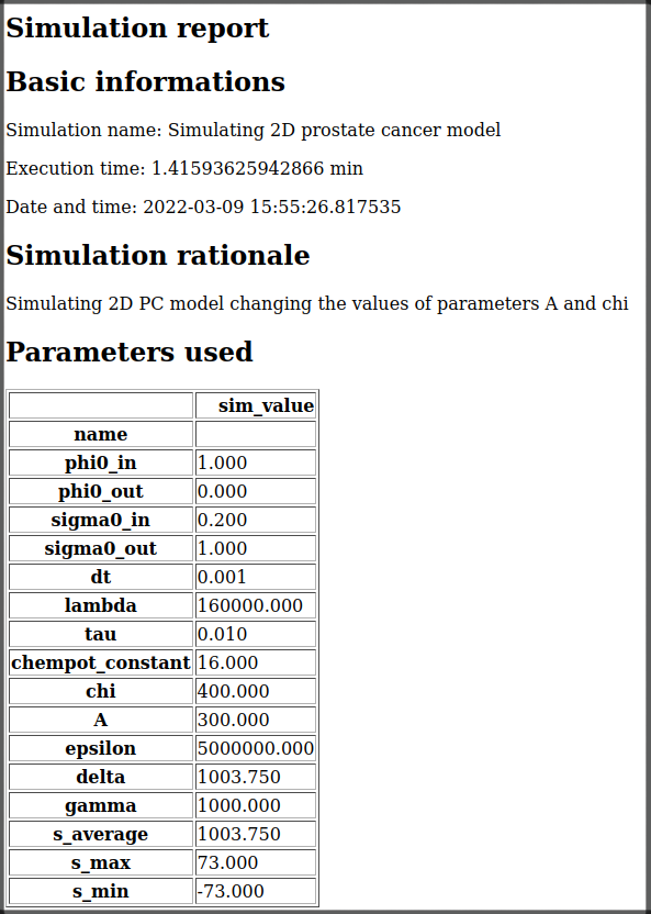
• At the end of the simulation, we use the method save_sim_info to store the simulation meta-data inside the data folder. Indeed, this method generates a file called sim_info.html, unique for each simulation, containing all the meta-data we asked to save. For instance, this is the file generated for the first simulation:

After the loop, the result will be stored in a tree like the following:

demo_out/multiple_pc_simulations/
├── 0000
│   ├── phi.h5
│   ├── phi.xdmf
│   ├── sigma.h5
│   ├── sigma.xdmf
│   └── sim_info.html
└── 0001
    ├── phi.h5
    ├── phi.xdmf
    ├── sigma.h5
    ├── sigma.xdmf
    └── sim_info.html

As you can see, there are two nested folders inside demo_out/multiple_pc_simulations, called 0000 (the first simulation) and 0001 (the second simulation). For each folder, the simulation output (phi.* and sigma.*) is stored together with the report file sim_info.html, containing the simulation meta-data.

Result

We uploaded on Youtube the result on this simulation. You can check it out below or at this link

Full code

import numpy as np
import fenics
import time
from tqdm import tqdm
from pathlib import Path
import petsc4py
from mocafe.fenut.solvers import SNESProblem
from mocafe.fenut.fenut import get_mixed_function_space, setup_xdmf_files
from mocafe.fenut.mansimdata import setup_data_folder, save_sim_info
from mocafe.expressions import EllipseField
from mocafe.fenut.parameters import from_dict
import mocafe.litforms.prostate_cancer as pc_model


def run_prostate_cancer_simulation(loading_message, parameters, data_folder):
    phi_xdmf, sigma_xdmf = setup_xdmf_files(["phi", "sigma"], data_folder)

    # Mesh definition
    nx = 130
    ny = nx
    x_max = 1000  # um
    x_min = -1000  # um
    y_max = x_max
    y_min = x_min

    mesh = fenics.RectangleMesh(fenics.Point(x_min, y_min),
                                fenics.Point(x_max, y_max),
                                nx,
                                ny)

    # Spatial discretization
    function_space = get_mixed_function_space(mesh, 2, "CG", 1)

    # Initial conditions
    semiax_x = 100  # um
    semiax_y = 150  # um
    phi0 = EllipseField(center=np.array([0., 0.]),
                        semiax_x=semiax_x,
                        semiax_y=semiax_y,
                        inside_value=parameters.get_value("phi0_in"),
                        outside_value=parameters.get_value("phi0_out"))
    phi0 = fenics.interpolate(phi0, function_space.sub(0).collapse())
    phi_xdmf.write(phi0, 0)

    sigma0 = EllipseField(center=np.array([0., 0.]),
                          semiax_x=semiax_x,
                          semiax_y=semiax_y,
                          inside_value=parameters.get_value("sigma0_in"),
                          outside_value=parameters.get_value("sigma0_out"))
    sigma0 = fenics.interpolate(sigma0, function_space.sub(0).collapse())
    sigma_xdmf.write(sigma0, 0)

    # Weak form definition
    u = fenics.Function(function_space)
    phi, sigma = fenics.split(u)

    s_exp = fenics.Expression("(s_av + s_min) + ((s_max - s_min)*(random()/((double)RAND_MAX)))",
                              degree=2,
                              s_av=parameters.get_value("s_average"),
                              s_min=parameters.get_value("s_min"),
                              s_max=parameters.get_value("s_max"))
    s = fenics.interpolate(s_exp, function_space.sub(0).collapse())

    v1, v2 = fenics.TestFunctions(function_space)
    weak_form = pc_model.prostate_cancer_form(phi, phi0, sigma, v1, parameters) + \
                pc_model.prostate_cancer_nutrient_form(sigma, sigma0, phi, v2, s, parameters)

    # Simulation: setup
    n_steps = 1000

    if rank == 0:
        progress_bar = tqdm(total=n_steps, ncols=100)
        progress_bar.set_description(loading_message)
    else:
        progress_bar = None

    petsc4py.init([__name__,
                   "-snes_type", "newtonls",
                   "-ksp_type", "gmres",
                   "-pc_type", "gamg"])
    from petsc4py import PETSc

    # define solver
    snes_solver = PETSc.SNES().create(comm)
    snes_solver.setFromOptions()

    t = 0
    for current_step in range(n_steps):
        # update time
        t += parameters.get_value("dt")

        # define problem
        problem = SNESProblem(weak_form, u, [])

        # set up algebraic system for SNES
        b = fenics.PETScVector()
        J_mat = fenics.PETScMatrix()
        snes_solver.setFunction(problem.F, b.vec())
        snes_solver.setJacobian(problem.J, J_mat.mat())

        # solve system
        snes_solver.solve(None, u.vector().vec())

        # save new values to phi0 and sigma0, in order for them to be the initial condition for the next step
        fenics.assign([phi0, sigma0], u)

        # save current solutions to file
        phi_xdmf.write(phi0, t)  # write the value of phi at time t
        sigma_xdmf.write(sigma0, t)  # write the value of sigma at time t

        # update progress bar
        if rank == 0:
            progress_bar.update(1)


# initial setup
fenics.set_log_level(fenics.LogLevel.ERROR)
comm = fenics.MPI.comm_world
rank = comm.Get_rank()

# get this file folder
file_folder = Path(__file__).parent.resolve()

# init standard parameters
std_parameters = from_dict({
    "phi0_in": 1.,  # adimentional
    "phi0_out": 0.,  # adimdimentional
    "sigma0_in": 0.2,  # adimentional
    "sigma0_out": 1.,  # adimentional
    "dt": 0.001,  # years
    "lambda": 1.6E5,  # (um^2) / years
    "tau": 0.01,  # years
    "chempot_constant": 16,  # adimensional
    "chi": 600.0,  # Liters / (gram * years)
    "A": 600.0,  # 1 / years
    "epsilon": 5.0E6,  # (um^2) / years
    "delta": 1003.75,  # grams / (Liters * years)
    "gamma": 1000.0,  # grams / (Liters * years)
    "s_average": 2.75 * 365,  # 961.2,  # grams / (Liters * years)
    "s_max": 73.,
    "s_min": -73.
})

# define parameters values to test
chi_values = [400, 600]
A_values = [300, 600]

# run multiple simulations
for chi_value, A_value in zip(chi_values, A_values):
    # set data folder for current simulation
    data_folder = setup_data_folder(folder_path=f"{file_folder / Path('demo_out')}/multiple_pc_simulations")

    # set new parameters values
    std_parameters.set_value("chi", chi_value)
    std_parameters.set_value("A", A_value)

    # run simulation measuring execution time
    init_time = time.time()
    run_prostate_cancer_simulation(f"simulating for chi = {chi_value}, A = {A_value}",
                                   std_parameters,
                                   data_folder)
    execution_time = time.time() - init_time

    # store simulation meta-data
    save_sim_info(data_folder,
                  parameters=std_parameters,
                  execution_time=execution_time,
                  sim_name="Simulating 2D prostate cancer model",
                  sim_description="Simulating 2D PC model changing the values of parameters A and chi")