A brief introduction to FEniCS

This demo is ment to give a brief introduction to the FEniCS computing platform for the Mocafe users who never came across this software. For a complete understanding of this demo it is required to have a basic understanding of partial differential equations (PDEs), finite element method (FEM), and Python scripting.

This demo is deliberately very brief, given the presence online of excellent and extensive tutorials. Just to mention a few, you can find for free the book The FEniCS Tutorial [LL17], a collection of documented demos, and the tutorial created by J. S. Dokken for the development version of FEniCS, FEniCSx. In case you feel the need of a more gradual introduction to FEniCS, we recommend you those websites.

What is FEniCS

FEniCS [ABH+15] is a popular open source computing platform for solving PDEs, mainly using the Finite Element Method. FEniCS provides high level Python and C++ interfaces together with access to powerful algebra backend, ensuring both efficiency and usability.

The basic FEniCS workflow

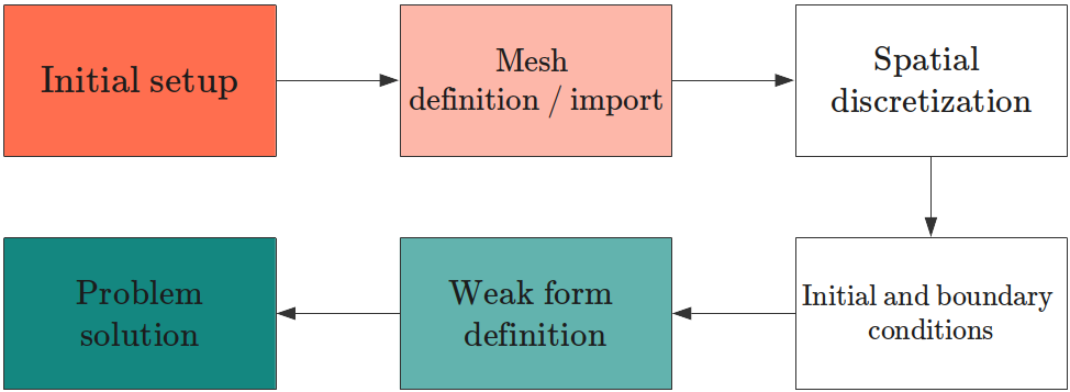
Every FEniCS script follows a general workflow to solve PDEs that is summarized in the following. See also the figure below for a brief summary

0. Initial setup. The operations here depend on the problem you’re solving but, in general, it is a good practice to define some general variables at the beginning of the script. Also, this might be the good place for setting up loggers, files to store data, and so on.

1. Mesh definition or import. Before solving any PDE problem, you need to define the space where you want to solve it. FEniCS has built-in methods to generate simple meshes, such as 2D rectangles or 3D cubes. However, it is also possible (and often more interesting) to import any given mesh (e.g. a 3D model of a gear).

2. Definition of the spatial discretization. Then, it is useful to define how you want your PDE to be discretized in space choosing the type of Finite Element to use. This might be a critical choice for some problems.

3. Definition of initial and boundary conditions.

4. Definition of the weak form. One of the greatest things in FEniCS is the Unified Form language (UFL) [AlnaesLOlgaard+14], which makes the coding of the PDE weak form very close to the mathematical language.

5. Problem solution. The actual solution of the PDE system. This might be an iteration in time, in case the PDE system you’re considering is time-dependent.

We’re going to see this very workflow in practice in the next section.

The diffusion (or heat) equation solved with FEniCS

The simplest time-variant PDE is the so-called diffusion equation (or heat equation) which is used both to describe the diffusion of a chemical in a fluid (e.g. salt in water) and the evolution of heat distribution in a conductor.

The equation reads:

\[ \begin{align}\begin{aligned}\begin{split}\frac{\partial u}{\partial t} = D \nabla^2 u & \quad \textrm{in} \; \Omega \\\end{split}\\\begin{split}u(t=0) = u_0 & \quad \textrm{in} \; \Omega \\\end{split}\\\begin{split}\nabla u \cdot n = 0 & \quad \textrm{in} \; \Gamma \\\end{split}\end{aligned}\end{align} \]

Where:

• the first row is the actual PDE, which is defined on the entire spatial domain \(\Omega\);

• the second row represents the initial condition (which will be discussed in detail below);

• and the third row represents the boundary condition (set to natural Neumann), which is of course defined on the boundary \(\Gamma\).

Solving this problem in FEniCS requires just a few lines of Python code. Let’s see the implementation in detail.

Initial setup

In this simple case we just import the FEniCS package and create an .xdmf file, which will used for storing the solution of our problem in time. You can open this kind of file with the software Paraview, which is one of the recommended ways to visualize results obtained with FEniCS.

import fenics

# create file
u_xdmf = fenics.XDMFFile("./demo_out/introduction_to_fenics/u.xdmf")

Mesh definition

Here we use one of the FEniCS builtin function to create a simple square mesh of side 1. Notice that you can specify the number of elements for each side (in this case, 32 x 32).

mesh = fenics.UnitSquareMesh(32, 32)

Spatial discretization

Then, we can choose how to approximate the solution of our PDE in space or, in FEM-terms, which kind of finite element we need for solving our problem. It is not simple to explain a few words what a finite element is; simply put, the kind of finite element specifies the class of piece-wise functions we want to use to approximate the solution of our PDE of interest.

However, choosing the kind of finite element to use is extremely simple with the FunctionSpace class in FEniCS. Below, with a single line of code, we generate the finite elements for our mesh, specifying that we want Lagrange elements of degree 1.

V = fenics.FunctionSpace(mesh, "Lagrange", 1)

Initial and boundary conditions

To clearly visualize the behaviour of the diffusion equation, we decided to have a simple circle as initial condition. Physically-speaking, this is like considering an initial situation where a chemical is all concentrated in a circle at the center of the domain.

To define this initial condition, we can use a so-called Expression, which is nothing more than a mathematical expression written in C++. If you understand the basics of C, you can see that the input of the following object is a C string defining a mathematical function, which is 1 inside a circle centered in (c_x, c_y), and 0 outside.

u_0_exp = fenics.Expression("(pow(x[0] - c_x, 2) + pow(x[1] - c_y, 2) <= pow(r, 2)) ? 1. : 0.",
                            degree=2,
                            c_x=0.5, c_y=0.5, r=0.25)

This Expression, however, is just a “symbolic” representation of our initial condition. In order to translate it in an actual function, discretized in space according to our problem, we need to project it in our function space.

FEniCS has a built in function to do so, which is called, indeed, project:

u_0 = fenics.project(u_0_exp, V)

Regarding the boundary condition, we need no code to implement natural Neumann conditions in FEniCS because it is the default setup. For different boundary conditions, you’re invited to check specific tutorials.

Finally, it is useful to store this initial condition in the .xdmf file we defined above, simply calling the method write(phi0, 0). The second argument, 0, just represent the fact that this is the value of the function at time 0. As we’re going to see in the simulation, the file phi_xdmf can collect the values of phi for each time.

t = 0
u_xdmf.write(u_0, t)

Weak form definition

The definition of the weak form of our PDE of interest is the starting point of the finite elment metod. Briefly, the weak form is just a mathematical problem, derived from the original PDE, of which solution is an approximation of our PDE of interest in a given function space \(V\).

For people experienced in weak form definition is very simple to derive the one for the diffusion equation. The discretization of the PDE in time with backward Euler leads to the following semi-discrete equation:

\[\frac{u - u_0}{dt} - D \nabla^2 u = 0\]

And the weak form of this problem can be written in the canonical form:

\[a(u, v) = L(v)\]

Where \(a\) and \(L\) are defined as:

\[\begin{split}a(u, v) & = \int_{\Omega} \frac{u}{dt} \cdot v \cdot dx + \int_{\Omega} D \cdot \nabla u \cdot \nabla v \cdot dx \\ L(v) & = \int_{\Omega} \frac{u_0}{dt} \cdot v \cdot dx \\\end{split}\]

In the following, we translate this mathematical equation into scientific code leveraging one of the best feature of FEniCS: the Unified Form Language (UFL). Indeed, you can see yourself that the definition of a and L is very close to the actual mathematical formula.

D = fenics.Constant(1.)
dt = 0.001
u = fenics.TrialFunction(V)
v = fenics.TestFunction(V)
a = (u / dt) * v * fenics.dx + D * fenics.dot(fenics.grad(u), fenics.grad(v)) * fenics.dx
L = (u_0 / dt) * v * fenics.dx

# From this code, FEniCS is able to efficiently construct all the data structures needed to get our
# solution at each time step. If you wank to know more about this topic, you are again encouraged to have a look to The
# Fenics Tutorial to start :cite:`LangtangenLogg2017`.

Problem solution

The last thing to do is to just solve our differential equation.

Since the equation is time-dependent, we need to iterate in time and solve for each time step the equation using the following for loop:

u = fenics.Function(V)
for n in range(30):
    # update time
    t += dt
    # compute solution at current time step
    fenics.solve(a == L, u)
    # assign new solution to old
    fenics.assign(u_0, u)
    # save solution for the current time step
    u_xdmf.write(u_0, t)

Notice that also here the flow is very basic:

• we update time;

• we call the FEniCS function solve to solve the equation (storing the result on the variable u);

• we assign the result to u_0 (for the following time step);

• and we store the solution to our .xdmf file.

However, this basic method should be used with care: it works perfectly with simple PDEs, but sometimes the “black-box” function solve is not the most efficient way compute our solution. In those cases, it is recommended to use more advanced techniques. In other tutorials we will show how to use different solution algorithms in FEniCS.

Below you can find an animation of the result of this script:

Full code

import fenics

# create file
u_xdmf = fenics.XDMFFile("./demo_out/introduction_to_fenics/u.xdmf")

mesh = fenics.UnitSquareMesh(32, 32)

V = fenics.FunctionSpace(mesh, "Lagrange", 1)

u_0_exp = fenics.Expression("(pow(x[0] - c_x, 2) + pow(x[1] - c_y, 2) <= pow(r, 2)) ? 1. : 0.",
                          degree=2,
                          c_x=0.5, c_y=0.5, r=0.25)
u_0 = fenics.project(u_0_exp, V)

t = 0
u_xdmf.write(u_0, t)

D = fenics.Constant(1.)
dt = 0.001
u = fenics.TrialFunction(V)
v = fenics.TestFunction(V)
a = (u / dt) * v * fenics.dx + D * fenics.dot(fenics.grad(u), fenics.grad(v)) * fenics.dx
L = (u_0 / dt) * v * fenics.dx

u = fenics.Function(V)
for n in range(30):
  # update time
  t += dt
  # compute solution at current time step
  fenics.solve(a == L, u)
  # assign new solution to old
  fenics.assign(u_0, u)
  # save solution for the current time step
  u_xdmf.write(u_0, t)