Local analysis
In this part of the demo, we continue the analysis on the SH3 domain example from the Protein Ensemble Database (PED) and highlight how the IDPET package can provide insights into local structural information from conformational ensembles. Specifically, this demo shows how to extract the following information:
Contact maps
Ramachandran plots
Alpha angle distribution
Relative DSSP through each ensemble (secondary structure)
Site-specific flexibility and order parameters
Initialize the analysis
Initializition of the analysis already described in the demo for the global analysis.
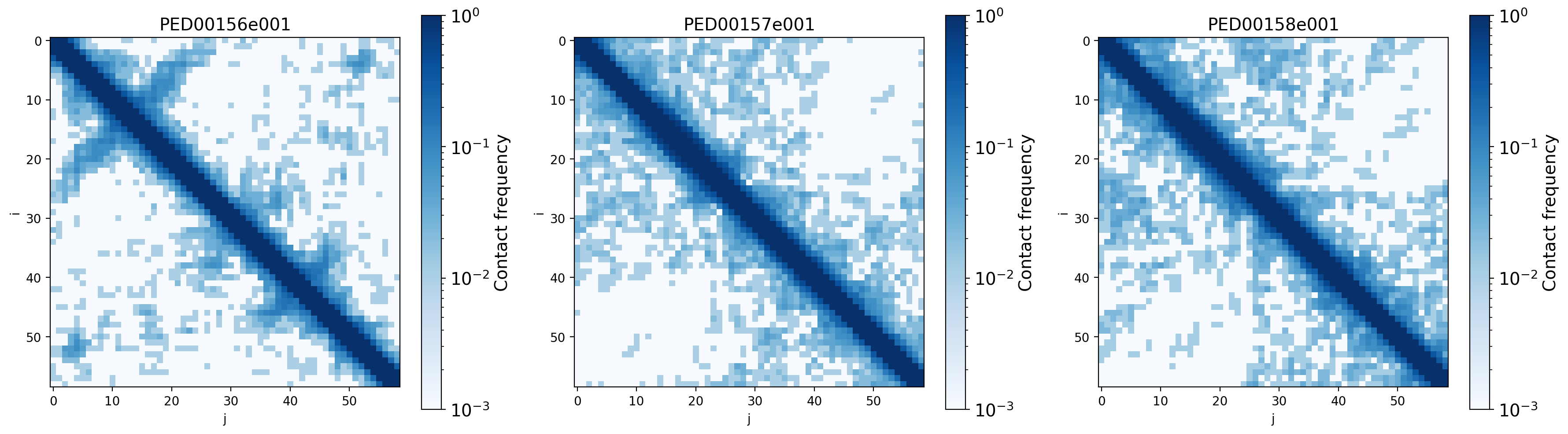
Contact probability map
The contact map is a graphical representation of the contact matrix, whose elements represent the likelihood of contact between two residues, with values approaching 1 indicating close proximity and values approaching 0 indicating spatial separation. The graphs show the contact maps generated from the coordinates of the alpha carbon atoms of the proteins under study, aiming to understand the spatial relationships and local interactions within the protein structure.
“log_scale”: If True, use a log scale range; default is True.
“avoid_zero”: If True, avoid contacts with zero counts by adding to all contacts a pseudo count of 1e-6
“threshold”: Determines the threshold for calculating the contact frequencies; default is 0.8 nm.
“dpi”: For changing the quality and dimension of the output figure; default is 96.
“save”: If True, the plot will be saved as an image file; default is False.
“color”: The colormap to use for the contact probability map. Default is ‘Blues’.
“ax”: A list or array of Axes objects to plot on; default is None, which creates new axes.
vis.contact_prob_maps(log_scale=True, threshold=0.7)
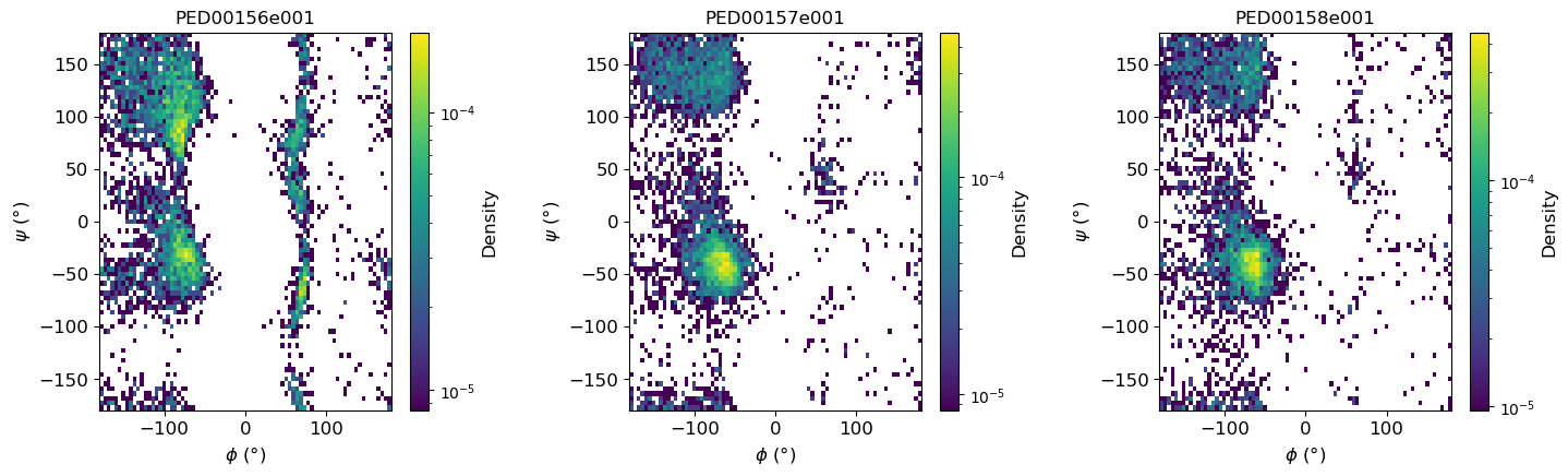
2D Ramachandran histograms
The function generates Ramachandran plots to visualize the distribution of phi (ϕ) and psi (ψ) torsion angles of proteins within the ensembles. To calculate the torsion angles, MDTraj functions are used, and the results are then converted to degrees using np.degrees. If two_d_hist is set to False, it returns a simple scatter plot for all ensembles in a single plot. If set to True, it returns a 2D histogram for each ensemble, where the angles are grouped into a 2D histogram showing the population density of the conformations.
“two_d_hist”: If True, it returns a 2D histogram for each ensemble. Default is True.
“bins”: You can customize the bins for 2D histogram. Default is (-180, 180, 80).
“log_scale”: If True, the histogram will be plotted on a logarithmic scale. Default is True.
“dpi”: The DPI (dots per inch) of the output figure. Default is 96.
“save”: If True, the plot will be saved as an image file in the specified directory. Default is False.*
“color”: The colormap to use for the 2D histogram. Default is ‘viridis’..
“ax”: The matplotlib Axes object on which to plot; if None, creates a new Axes object.
vis.ramachandran_plots(two_d_hist=True)
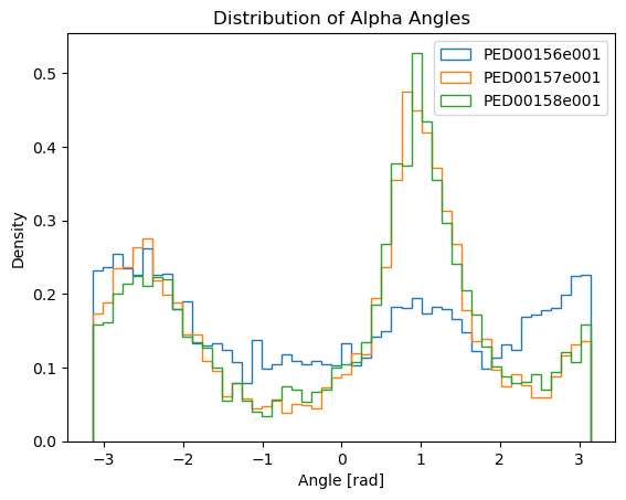
Alpha angles dihedral distribution
Alpha angles are a specific type of dihedral angle calculated using the C-alpha (Cα) atoms of a protein backbone. A dihedral angle, also known as a torsion angle, is the angle between two planes formed by four sequentially bonded atoms, providing insight into the 3D conformation of the molecule.
To calculate alpha angles, the indices of all Cα atoms in the protein are identified, and sets of four consecutive Cα atoms are grouped. Using these groups, the torsion (dihedral) angles are computed with the MDTraj function, which takes the trajectory and a list of tuples containing the indices of the four Cα atoms. The output is a numpy array with the dihedral angles for each set, representing the alpha angles that provide important insights into the protein’s three-dimensional structure and dynamics.
“bins”: Number of bins for the histogram; default is 50.
“save”: If True, saves the plot in the data directory; default is False.
“ax”: The matplotlib Axes object on which to plot; if None, creates a new Axes object.
vis.alpha_angles()
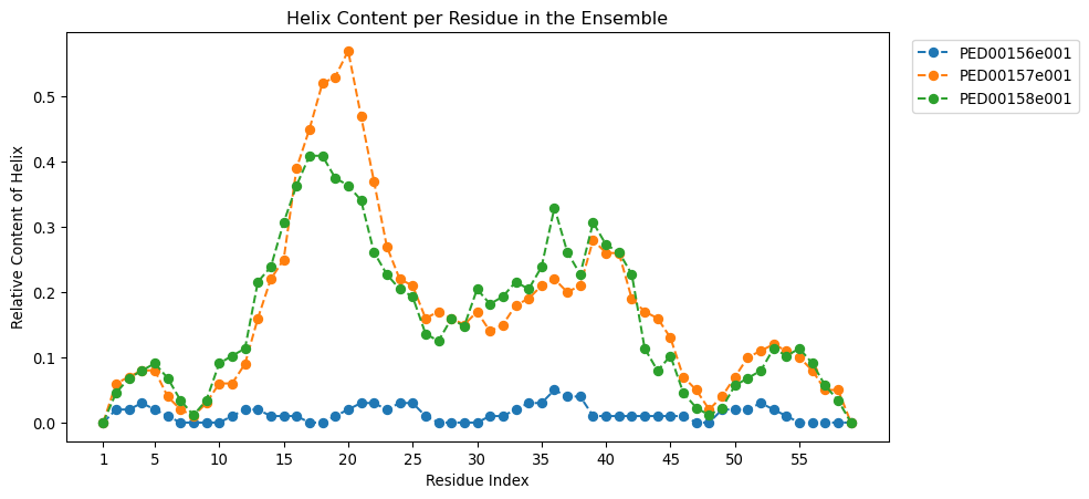
Relative DSSP (Dictionary of Secondary Structure of Proteins) content
This function visualizes the relative content of a selected secondary structure type (helix, coil, or strand) for each residue across multiple protein ensembles. It retrieves the DSSP data for all ensembles and plots, for each residue position, the fraction of conformers adopting the chosen secondary structure.
The relative content for residue i and DSSP type d is calculated as:
where:
\(R_i(d)\) — relative content of secondary structure type d at residue i
\(N_i(d)\) — number of conformers in which residue i is assigned DSSP code d
\(N_{\\text{conf}}\) — total number of conformers in the ensemble
A value of \(R_i(d) = 1\) indicates that the residue always adopts the specified secondary structure, while \(R_i(d) = 0\) means it never does. Intermediate values represent partial occupancy, reflecting structural heterogeneity across the ensemble.
Note
This analysis is not applicable to coarse-grained models.
parameters:
“dssp_code”: The selected dssp code , it could be selected between ‘H’ for Helix, ‘C’ for Coil and ‘E’ for strand. It works based on the simplified DSSP codes.
“dpi”:The DPI (dots per inch) of the output figure. Default is 96.
“auto_xticks”:If True, use matplotlib default xticks.
“xtick_interval”:If auto_xticks is False, this parameter defines the interval between displayed residue indices on the x-axis. Residue 1 is always included,followed by every xtick_interval residues (e.g., 1, 5, 10, 15 if `xtick_interval`=5).
“figsize”:The size of the figure in inches. Default is (10, 5).
“save”:If True, the plot will be saved in the data directory. Default is False.
“ax”: The matplotlib Axes object on which to plot; if None, creates a new Axes object.
vis.relative_dssp_content(dssp_code ='H')
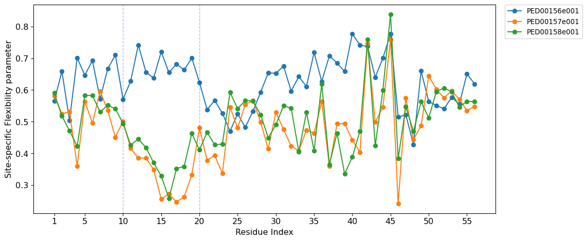
Site-specific Flexibility Parameter
The site-specific flexibility parameter quantifies the local flexibility of a protein chain at each residue. It ranges from 0 (high flexibility) to 1 (no flexibility). If all conformers have identical dihedral angles at a residue, the circular variance equals one, indicating no flexibility. Conversely, for a large ensemble with a uniform distribution of dihedral angles, the circular variance tends toward zero.
The site-specific flexibility parameter is defined using the circular variance of the Ramachandran angles \(\phi_i\) and \(\psi_i\). The circular variance of \(\phi_i\) is given by:
An analogous expression applies for \(R_{\psi_i}\). The site-specific flexibility parameter \(f_i\) is then defined as:
This parameter describes the dispersion of backbone dihedral angles (\(\phi\), \(\psi\)) for each residue and is conceptually similar to the dihedral angle order parameter originally introduced by Hyberts and Wagner [1]. Both quantify how narrowly distributed local torsion angles are across an ensemble, differing mainly in scale—Hyberts’ order parameter measures structural order directly, whereas Jeschke’s flexibility parameter expresses its inverse (i.e., disorder).
The implementation in IDPET follows the formulation proposed by Jeschke [2], who also introduced the site-specific order parameter (next section) to describe the orientational correlation of backbone segments along the entire chain. This complementary measure captures how persistently local chain orientations are maintained across conformers, thereby extending the concept of local dihedral order to characterize global backbone orientational order within an ensemble.
parameters:
“dpi”:The DPI (dots per inch) of the output figure. Default is 96.
“auto_xticks”:If True, use matplotlib default xticks.
“xtick_interval”:If auto_xticks is False, this parameter defines the interval between displayed residue indices on the x-axis. Residue 1 is always included,followed by every xtick_interval residues (e.g., 1, 5, 10, 15 if `xtick_interval`=5).
“figsize”:The size of the figure in inches. Default is (10, 5).
“save”:If True, the plot will be saved in the data directory. Default is False.
“ax”: The matplotlib Axes object on which to plot; if None, creates a new Axes object.
vis.site_specific_flexibility(pointer=[10,20], figsize=(12, 5),auto_xticks=False ,xtick_interval=5, save=True);
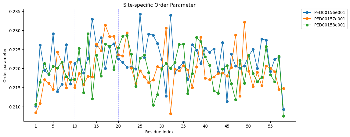
Site-specific order parameter
The “Site-specific order parameter” is an indicator that evaluates the local order within a protein chain. This parameter measures the orientation correlation between neighboring residues along the protein chain, based on the direction of the Cα-Cα vectors. The parameter is derived by computing the ensemble mean of the cosine of the angle between these vectors and assessing its variance across conformers.
The mean orientation correlation \(<cos \theta_{ij}>\) is calculated as:
Where:
\(w_c\) is the weight of conformer \(c\)
\(C\) is the total number of conformers
\(cos \theta_{ij,c}\) is the cosine of the angle between vectors \(r_{i,i+1}\) and \(r_{j,j+1}\) for conformer \(c\).
The variance \(<\sigma_{ij}^2>\) of \(<cos \theta_{ij}>\) is given by:
The site-specific order parameter \(K_{ij}\) is defined as:
To characterize the order at residue \(i\) in relation to the entire chain, the site-specific order parameter \(o_{i}\) is computed by summing \(K_{ij}\) over all residues \(j\) :
where \(N\) represents the total number of residues in the protein chain.
parameters:
“dpi”:The DPI (dots per inch) of the output figure. Default is 96.
“auto_xticks”:If True, use matplotlib default xticks.
“xtick_interval”:If auto_xticks is False, this parameter defines the interval between displayed residue indices on the x-axis. Residue 1 is always included,followed by every xtick_interval residues (e.g., 1, 5, 10, 15 if `xtick_interval`=5).
“figsize”:The size of the figure in inches. Default is (10, 5).
“save”:If True, the plot will be saved in the data directory. Default is False.
“ax”: The matplotlib Axes object on which to plot; if None, creates a new Axes object.
vis.site_specific_order(pointer=[10,20],auto_xticks=False,xtick_interval=5 ,figsize=(12, 5), save=True);